ANOVAs are kinda cool!
Today in ecology lab, I learned how to run an Analysis of Variance (ANOVA)! The specific type of ANOVA I learned how to use is the Kruskal-Wallis test. It is nonparametric and doesn’t depend on a normal distribution, so we used it. I later learned it is used to compare medians. The Kruskal-Wallis test is ranked, which means that for each factor, a numerical integer is assigned based on how high or low it is relative to the others in the data set, and then you calculate the sum of ranks for each group to get an H-statistic, which is pretty similar to a chi-square value.
The Experiment
To run our ANOVA we had data about plants: Last week, we had gone out in the field and collected goldenrod plants. The goldenrod plant is a very unassuming plant. We collected them from places around UMass and we tried to note what environmental factors they were exposed to.
Usually the Teaching Assistant helps us aggregate the data but she wasn’t there because she was trying to get a fellowship :) ! So, that meant that I had to aggregate the data. It was stressful being that responsible, but it also wasn’t too bad - just a lot of copying and pasting. We also had drop-down menus for factors so people didn’t just write their own, which is what happened last time. (The problem was solved by a nightmare script that’s 100 lines long and exports several .CSV files because I couldn’t figure out how to use _fulljoin() in dplyr. Whoops!). The good thing about being responsible for aggregating the data was that I got to name the variables what I liked and use snake instead of having to rewrite the headings later. Haha!
Anyway, here’s the data for what we worked on in the lab.
head(plants)
## # A tibble: 6 x 14
##   group_number plant_number total_plant_hei~ height_lowest_l~
##   <chr>               <dbl>            <dbl>            <dbl>
## 1 Yellow Team             1              79               0
## 2 Yellow Team             2              87               6
## 3 Yellow Team             3             140              10
## 4 Yellow Team             4             123              16.5
## 5 Yellow Team             5             115              14
## 6 Yellow Team             6             124.             12
## # ... with 10 more variables: height_lowest_flower <dbl>,
## #   number_leaves <dbl>, weight_leaves <dbl>, weight_flowers <dbl>,
## #   weight_stem <dbl>, habitat <chr>, average_plant_stand_height <dbl>,
## #   exposure <chr>, moisture_level <chr>, habitat_type <chr>
When working in groups we had to test whether the habitat might have impacted some element of the plant’s physiology from our collected variables. To do this, our group specifically wanted to test the effect of habitat on how the plant allocates its energy. For example, we decided to compare plants that were living in a saline environment near the shoreline versus plants that were living in a grassy environment. We wanted to see if this effected their stem length, leaf count, and other things.
Cleaning the Data
To clean the data, I selected only the groups that had collected from saline and grassland environments. This broke down nicely by team name so that’s what I used. However, this could’ve been a source of error becacuse of measurement error being different between the two groups - splitting up half and half groups collecting from both shoreline and grassy environments might have reduced this, but would’ve been much more complicated logistically.
plants2 <- plants %>%
  mutate(ratio_stem = number_leaves/total_plant_height) %>%
  filter(group_number == "Treehuggers" | group_number == "Dennis")
ANOVAs and Graphs
Here are the results! For the first hypothesis we wanted to test whether the plant height differed by what habitat it was collected from. You can see these box plots are super different from each other, so it’s no surprise that the H-statistic was so high and the p-value so small and significant.
ggplot(plants2, aes(habitat_type, total_plant_height, fill=habitat_type)) +
  scale_fill_manual(values=c("lightgreen", "skyblue")) +
  geom_boxplot() +
  labs(x="Habitat Type", y="Total Plant Height", title = "Boxplot of Plant Height by Habitat Type")
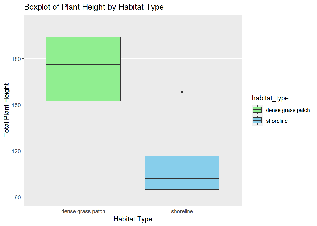
kruskal.test(total_plant_height ~ habitat_type, plants2) # p value 3.674 e-5
##
## 	Kruskal-Wallis rank sum test
##
## data:  total_plant_height by habitat_type
## Kruskal-Wallis chi-squared = 17.033, df = 1, p-value = 3.674e-05
For the second hypothesis we wanted to test whether the number of leaves differed by what habitat it was collected from. Again, these box plots are super different from each other, so again we see a high H-statistic and small p-value.
ggplot(plants2, aes(habitat_type, number_leaves, fill= habitat_type)) +
  scale_fill_manual(values=c("lightgreen","skyblue")) +
  geom_boxplot() +
  labs(x="Habitat Type", y="Number of Leaves", title = "Boxplot of Number of Leaves by Habitat Type")
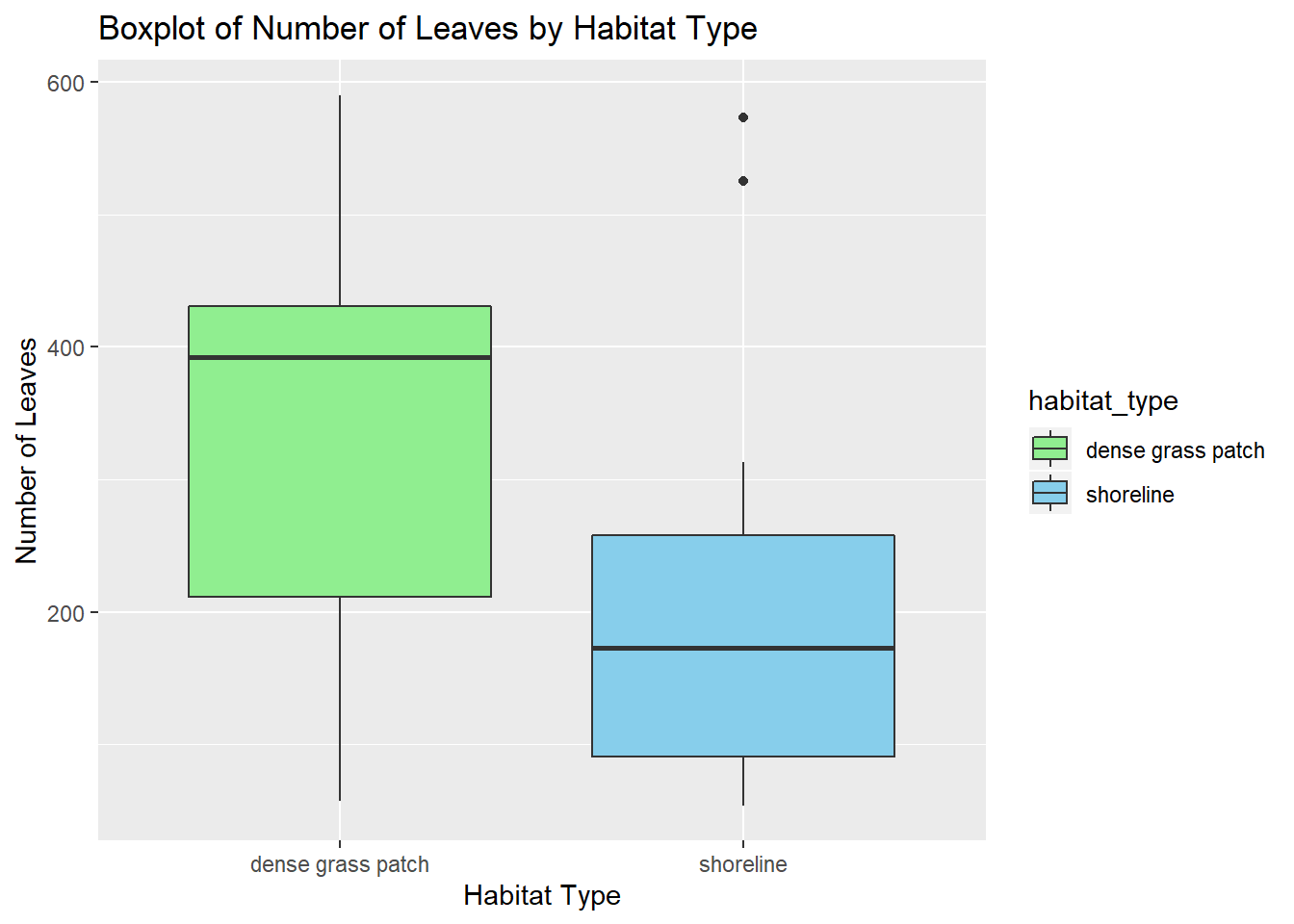
kruskal.test(number_leaves ~ habitat_type, plants2) # p value .02
##
## 	Kruskal-Wallis rank sum test
##
## data:  number_leaves by habitat_type
## Kruskal-Wallis chi-squared = 5.2994, df = 1, p-value = 0.02133
Lastly, we wanted to test whether the ratio of the stem to leaves by habitat were significantly different. I had gotten the stem and leaf ratio by using the mutate() function in dplyr and it’s included in the data cleaning above. We didn’t find that this statistically significant, which makes sense because not only are the medians pretty similar.
ggplot(plants2, aes(habitat_type, ratio_stem, fill=habitat_type)) +
  scale_fill_manual(values=c("lightgreen","skyblue")) +
  geom_boxplot() +
  labs(x="Habitat Type", y="Ratio of Number of Leaves to Stem Height", title = "Boxplot of Ratio of Number of Leaves to Stem Height by Habitat Type")

kruskal.test(ratio_stem ~ habitat_type, plants2) # p value .7244
##
## 	Kruskal-Wallis rank sum test
##
## data:  ratio_stem by habitat_type
## Kruskal-Wallis chi-squared = 0.1243, df = 1, p-value = 0.7244
The End
Learning how to do one kind of ANOVA in R was really fun and the Kruskal-Wallis test was pretty easy to understand and interpret. I’m glad we didn’t have to do the math by hand. A lot of people weirdly seemed to leave the lab without analyzing the data first, and don’t seem to be familiar with R so they might have to run it online or, God forbid, calculate thirty variances by hand for whatever hypothesis they’re testing. I prefer analyzing the data in the lab time so I can ask for help. My group actually worked super productively and we finished our entire team presentation before we left (which is awesome, so we don’t have to do it at home now.) Either way - a fun way to spend a Wednesday playing with R!