Ever since I’ve started this blog, I’ve been a huge fan of text mining. And I mean literal text mining, such as this sweet sentiment analysis a man made of him and his girlfriend’s text messages. I realized that my friend and I had been chatting for over a six months everyday through Facebook Messenger, and jumped at the chance to make some fun word clouds.
I’m going to show the code I wrote to make these graphs, but a lot of it was really difficult and mostly scraped from StackOverflow and again, Julia Silge’s awesome resource on Tidytext. So instead of subjecting you to seeing the output of said code, I’m presenting it, but have commented it out because the workflow is pretty awful. But sometimes, that’s how it be.
Downloading the data
Getting the data wasn’t that hard. I simply requested a log of my chats from Facebook, which asked me if I wanted to download the files as HTML or .JSON format. I ended up picking .JSON because someone on StackOverflow said to. It took a few minutes for the Facebook gods to give me my data in the form of a 247MB zipped file. When they did, I was surprised at how detailed they were - I had every message I’ve ever had with anyone on Facebook. In addition, they had even saved every image, gif, and file I’ve ever sent.
Reading in the data
Reading in the data was kind of challenging. I’ve never worked with .JSON files before. Luckily, there is a package for that called rjson.
Then, I did a ton of data cleaning. The first problem was that there was two different messages scripts. My friend and I have exchanged 20,000 messages, which is apparently too large to be contained in just one file. The .JSON files, which I’ve never technically worked with before, were read into R as lists, so I had to unlist everything, and then merge them together.
# library(tidyverse)
# library(rjson)
# library(tidytext)
# library(wordcloud)
# options(stringsAsFactors = FALSE)
#
# #putting json file into r
# messages <- fromJSON(file="C:/Users/chfal/Documents/GRAPH_MY_UNDERGRAD/message_1.json")
# messages2 <- fromJSON(file="C:/Users/chfal/Documents/GRAPH_MY_UNDERGRAD/message_2.json")
#
# #for each emessage i want: sender_name, content. time stamp would be cool, but for now, we are keeping it simple stupid
#
Then, I cleaned and subsetted the messages and removed stop words.
# #cleaning, subsetting
# class(messages)
#
# message2 <- messages$messages
# message3 <- messages2$messages
#
#
# #not exactly sure what this is going to do, but it works
# combined_messages <- rbind(message2,message3)
# mystery <- as.data.frame(do.call(rbind, combined_messages))
#
# #here are some stop words, i think there may be bugs in how things are defined as "words" in the process because i don't think either of us had typed just "?" by itself for example, and i think file names are read too hence png/jpg
#
# mystopwords <- tibble(word=c("?","?","?","bengreen_70fc0z5vcq", "png", "jpg", "yeah"))
After I cleaned and removed stop words, I separated the messages out by who had sent them.
#
# #cleo's messages and unnested tokens
# chf_messages <- messages_cleaned %>%
#   subset(messages_cleaned$sender_name =="Cleo Falvey")
#
# unlisted_messages_chf <- unlist(chf_messages$content) %>%
#   as.tibble()
#
# chf_unnested_tokens <- tidytext::unnest_tokens(unlisted_messages_chf, word, value)
#
# chf_words_in_counts <- chf_unnested_tokens %>%
#   anti_join(stop_words) %>%
#   anti_join(mystopwords) %>%
#   count(word, sort=TRUE)
#
# #ben's messages and unnested tokens
#
# bg_messages <- messages_cleaned %>%
#   subset(messages_cleaned$sender_name=="Ben Green")
#
# unlisted_messages_bg <- unlist(bg_messages$content) %>%
#   as.tibble()
#
# bg_unnested_tokens <- tidytext::unnest_tokens(unlisted_messages_bg, word, value)
#
# bg_words_in_counts <- bg_unnested_tokens %>%
#   anti_join(stop_words) %>%
#   anti_join(mystopwords) %>%
#   count(word, sort=TRUE)
After that, I was able to make my wordclouds! I used the wordcloud package in R. The hardest thing was honestly figuring out what the scale should be. The scale argument is supposed to be a vector that helps size and wrap the words proportional to their frequency. It didn’t do that very well, so I ended up guestimating the values until the text sort of wrapped and didn’t cut off any of the longer words.
# wordcloud(words = bg_words_in_counts$word, freq=bg_words_in_counts$n, max.words=50, random.order=FALSE, rot.per=.35, colors=brewer.pal(8,"Dark2"), scale=c(.1,1.5))
#
# wordcloud(words = chf_words_in_counts$word, freq=chf_words_in_counts$n, max.words=50, random.order=FALSE, rot.per=.35, colors=brewer.pal(8,"Dark2"),scale=c(.1,1.5))
Here are the results!
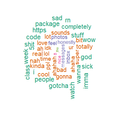
Figure 1: My Friend’s Most Common Words
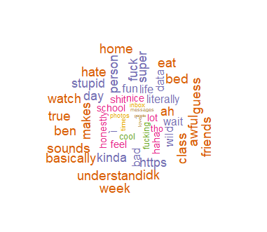
Figure 2: My Most Common Words
Most Interesting Results
I think the most interesting thing was seeing which were the most common words in our chat. After the classic stop words, our most common word was both “yeah” - which I removed in my analysis because it occurred at a frequency of 300 times, much larger than all the other words. Clearly we’re two agreeable people - just texting “yeah” back and forth to each other. Other themes that made me laugh was my friend’s quite common words included “code,” “package,” and “vim.” I’m a little disappointed in my own predisposition to swearing - not one, but two swear words appeared in my word cloud. It did look like I used more negative words - “hate,” “stupid,” “awful.”
I’m planning on presenting more graphs (bar/column, most likely) based on these chat conversations and performing more sentiment analysis. What I’d ideally like to do is create an automated pipeline that takes my Facebook messages and sends them to an ever-updated Shiny, because my friend and I have continued our conversation both during and after the creation of these graphs, but that’s probably a long way off based on my current limited coding experience.
Stay tuned for more sentiment analysis later, though!